Logistic regression in vaccine testing

I guess almost every scientist is familiar with linear regression and has already spent quite some time using it for various assays like BCA or Bradford assay for protein concentration determination. Nevertheless, probably not so many might have applied logistic regression, although this analysis is quite common for assays leading to quantal response data. Quantal response means that the outcome is of the form: response / no response, e.g. response, if the corresponding animal is alive, and no response, if the corresponding animal has died. In fact, the outcome $Y$ of these types of assays, that are also often referred to as dichotomous assays, is binary and often coded by 0 and 1. The independent variable is typically concentration or dose in those assays. Please note that logistic regression is most often performed with multiple independent variables especially in other disciplines. However, in this blogpost we will limit ourselves to the simplest case of only one independent variable $X$ . As we will see below, logistic regression is somehow related to linear regression, as both can be treated within the generalized linear model (GLM) framework (more on the basics of GLM, see also this blog post: Most European countries did not show exceptional excess mortalities during SARS-CoV-2 pandemic). If we assume that the outcome response has a probability of p to occur and if we assume the data is binomial, then the probability to have no response is $1-p$ . Logistic regression now models the logarithm of the so-called odds (ratio) $p/(1-p)$ in terms of a linear function:

$\ln{\left(\frac{p}{1-p}\right)}=\beta_0+\beta_1 X$

Maybe one more word concerning odds. Odds can be easily converted to probabilities if you prefer thinking in terms of those. Say our odds ratio is $O\equiv\frac{p}{1-p}$ , then we can calculate the probability of a response p simply by the following formula:

$p=\frac{O}{1+O}$

So, we could rewrite the equation above:

$\ln{\left(O\right)}=\beta_0+\beta_1X$

And solve for the odds:

$O=e^{\beta_0+\beta_1X}$

If we use the formula for the relation between the odds and the probability of a response, we end-up with:

$p=\frac{e^{\beta_0+\beta_1X}\ }{1+e^{\beta_0+\beta_1X}\ }=\frac{1}{1+e^{-\left(\beta_0+\beta_1X\right)}\ }$

The corresponding curve of $p$ vs. $X$ has a sigmoid-like shape and is essentially the fit curve that is often plotted together with the binary data or with corresponding probabilities (more on this below). In GLM terms this function is also known as the inverse link-function.

Let us now come to an example on how to perform logistic regression within the vaccine testing framework. Let’s say we have developed a new vaccine against the tetanus toxin and would like to compare its efficacy against a standard vaccine that is already commercially available, and which has a median effective dose of 2.5 IU/ml (i.e. international units per milliliter). The vaccine testing is done on guinea pigs (sorry, but unfortunately that is how it is done). The vaccine is applied to these animals in different doses (each animal only gets a single dose) and after some time the same animals become challenged with a certain amount of tetanus toxin. Animals which got very low doses of the vaccine are likely to die after they got the toxin administered, while those animals that got a higher vaccine dose are more likely to survive. The following table presents the results of the imaginary vaccine test.

dose	n	r
1	10	0
1.6	11	3
2.6	10	6
4.1	11	9
5.6	10	10

Herein denotes $n$ the total number of animals tested at the corresponding dose and $r$ denotes the number of guinea pigs that survived the toxin administration. For every single guinea pig the outcome or (let’s say) the response of the experiment is either dead or alive. If this is coded with 0 and 1, we could make a plot that looks like the following one:

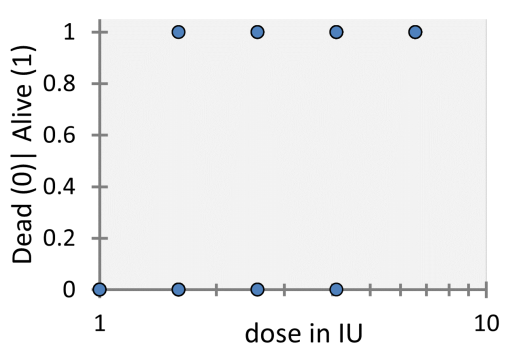
While these kinds of plots are common for logistic regression, in our case this plot is not appropriate as it does not show the number of underlying datapoints (since they overlap), so in this case it is more common to plot the probability of survival, i.e. the ratio $r/n$ versus the dose as shown in the following figure:

Logistic regression will find the optimal parameters $\beta_0$ and $\beta_1$ using a maximum likelihood approach and with those at hand one can calculate the ED₅₀as will be shown below. In between you might ask yourself the question: “Why not using a least-square regression approach?”. Because the response variable is binomial and thus, least-square regression does not apply, as it is applied to continuous data with normally distributed residuals. Back to maximum-likelihood estimation of $\beta_0$ and $\beta_1$ . The overall likelihood of the parameters $\beta_0$ and $\beta_1$ given that specific data $\left{y_i\right}_{i=1}^N$ is:

$\mathcal{L}\left(\beta_0,\beta_1|\left{y_i\right}_{i=1}^N\right)=\prod_{i=1}^{N}{p^{y_i}\left(1-p\right)^{1-y_i}}$

Where $y_i$ is either zero or one. Please note that these $y_i$ can be created for the data in the table shown above by breaking things down on to the single animal level. So, let us expand the data from the table above and convert the data to binary data:

Dose	1	1	1	1	1	1	1	1	1	1	1.6	1.6	1.6	1.6	1.6	1.6	1.6	1.6	1.6	1.6	1.6	…
y	0	0	0	0	0	0	0	0	0	0	0	0	1	0	1	0	0	0	0	0	0	…

I just wrote the $y_i$ up to the 2^nd dose, but it continuous up to the 5^th dose in a similar way (I used 5 doses here as you will see on my Excel-Sheet downloadable from the software page). By the way, it is quite common to use log-dose values instead of the linear dose values which I also did.
Maximizing the likelihood is equal to minimizing the negative likelihood. In Practice it better to maximize the log-likelihood or to minimize the negative log-likelihood as this prevents numerical overflows. The negative log-likelihood $\ell$ (that I personally prefer) becomes a summation of terms instead of a product:

$\ell\left(\beta_0,\beta_1|\left{y_i\right}_{i=1}^N\right)=-\left[\sum_{i=1}^{N}{y_i\ln{p}+\sum_{i=1}^{N}{\left(1-y_i\right)\ln{\left(1-p\right)}}}\right]$

In general, minimizing the negative log-likelihood needs to be done iteratively, e.g. using the Solver in Excel as is shown in a corresponding Excel-Sheet that you can find on our software page. Once the iteration succeeded and the parameters $\beta_0$ and $\beta_1$ are determined, we can now estimate the log of the median effective dose ED₅₀:

$\log\left(ED_{50}\right)=-\frac{\beta_0}{\beta_1}$

or (in its non-logarithmic form):

$ED_{50}=\exp\left(-\frac{\beta_0}{\beta_1}\right)$

If $X$ were log-dose values.

For the example data we obtain an ED₅₀ of about 2.3 IU/ml which is slightly lower than the 2.5 IU/ml of the reference vaccine. To compute a confidence interval for the ED₅₀ becomes a tedious task in Excel but is a common output of dedicated software packages (e.g. GraphPad Prism). In our case the 95 % confidence interval is [1.9081, 2.8605], so rather broad and ED50-value of the reference vaccine falls within this interval. So, we cannot claim the ED₅₀-difference to be significant at this point. Finally, the following figure shows the probability data, the corresponding fit curve (orange) and the ED₅₀-value (blue arrow).

Please have a look at the Excel-sheet that goes through the calculations step-by-step, so you get used to applying logistic regression.

Potency estimation (expressed in terms of the difference of ED50-values) of one or more vaccine candidates compared to a reference vaccine is often performed using parallel-line assays. Using a logistic model, the response / no response data of the reference vaccine and the test vaccine(s) is fitted globally (i.e. with shared slope $\beta_1$ but different intercepts $\beta_0$ for each data set). This can also be done quite easily in Excel as well. But I guess it might be better to demonstrate this in a video tutorial in near future.

Logistic regression in vaccine testing

Dr. Mario Schneider

Leave a Reply Cancel reply

Data analysis for scientists,
engineers and practitioners

Dr. Mario Schneider

You Might Also Like

Analysis of Bioassays

Don’t get fooled again by the R-squared

Leave a Reply Cancel reply