Do you agree with the following statement?
- An R² of 0.995 is very good.
- An R² value of -0.145 is impossible, since a squared value cannot be negative.
- A fit model resulting in an R² of 0.998 is preferred over another fit model giving an R² of 0.9134.
If you agreed to one of these statements, please go on reading. In this post I will show that all these statements are not true per se.
Natural scientists are often used to R² values above 0.900 which is due to the fact that their systems under investigation (e.g. particles, molecules, cells, etc.) can often be modelled and predicted more precisely than in research areas dealing with more complex system such as humans. Here, R² values below 0.5 are very common. While a quantum system can only assume a few discrete states, humans can assume an almost infinite number of states leading to very scattered results and thus to low R² values. Thus, statement (1) is not always true.
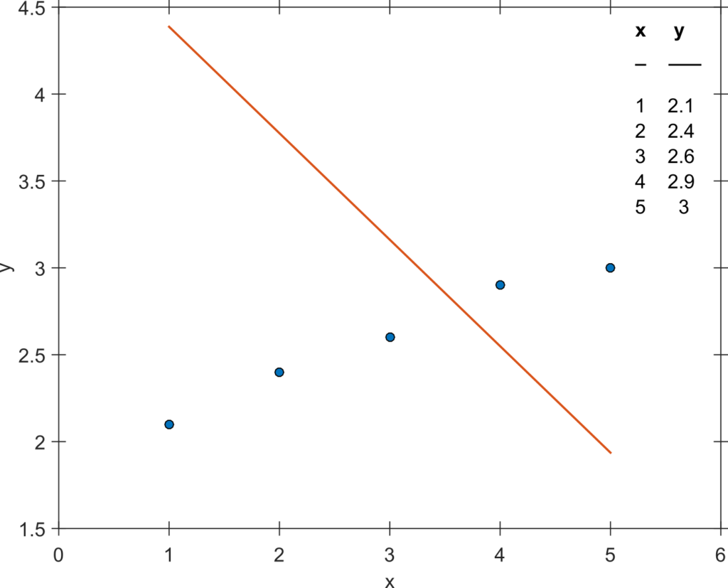
The first part of statement (2) is only true for linear regression with unconstrained fit parameters. However, if you fit the data in Figure 1 with a linear model of the form in which is the slope and 5 is the intercept that is constrained to 5, you will encounter that the R² becomes negative (about -15 in this example, please go ahead and try it).
Similarly, when multiple curves are fitted with shared parameters it might occur that some curves are almost perfectly fitted while for others the fit line is not even near the data points. The R² values of the latter curves might become negative, too. But isn’t it surprising that a value called “R squared” can become negative? This is due to the fact that R² is (in general) not calculated as the square of some other variable. At this point it is interesting to note that there are even multiple formulas published for calculating an R². Nevertheless, the most common one, I would say, is the following:

Herein  denotes the sum-of-squared residuals (sum of the squared vertical distance of the data points from the theoretical curve) and
  denotes the (total) sum-of-squared distances of the data points from the mean of the data. If the ratio in the equation above becomes negative, the R² value can become negative. As we have seen above, this might occur if an inappropriate fit model is used.
Statement (3) is rarely true in practice. A correct model could lead to a low R² value simply due to strong scattering of the data but still it would be the right model. A wrong model could lead to a high R² value but would still be the wrong model. On the other hand, completely different data sets might lead to equal R² values while applying the exact same fit model to each data set as impressively shown by Anscombe. The core of looking at this data set quartet is to look at the resulting graphs of data and fit line to prevent being flawed by the corresponding R² value.

While the first data set (top left) is reasonably well-fitted, the second one (top right) is rather paraboloid and not linear. The third data set (bottom left) contains an outlier erroneously shifting the regression line upwards. A robust regression could be applied in this case. The fourth data set (bottom right) shall illustrate that a single data point out of a group of data points can make the difference between correlation (R² = 0.67) and no correlation (R² = 0).
The R² shall in general not be used for model comparisons. If you would, for instance, compare a four parameter logistic function with a five parameter logistic function, the latter one will almost always have an R² closer to 1 due to the additional fit parameter which makes the theoretical curve cling closer to the data points and thus make the residuals smaller. Model comparison should rather be done with an F-test (if one model is a special-case of the other), on the Akaike information criterion or based on Bayesian model comparison using the evidence for instance.
I am not radically against the use of R² as a measure of fit quality (a term that you should define on your own). I look at it for instance when I know the correct model (e.g. the Lambert-Beer-Law which is a linear model) and I want to screen for “unusual data sets“ (those with low R² values) to draw conclusions about wrong instrument settings that might have caused these sets.
