What are confidence and prediction bands?
The moment a scientist starts working experimentally, the outcomes are prone to random error that mostly cannot be avoided (e.g. imperfections of instruments etc.). Say we measure an absorbance signal ( ) that is detected by a spectrophotomerter for various samples with different concentrations (
 ) of absorbing molecules. Due to instrument imperfections (detector noise etc.) the absorbance values will not be exactly the same for repetetive measurements but will slightly vary. This variability is often randomly distributed and approximately normal (central limit theorem). If we plot the signal versus concentration in a graph, the data points will approximately follow a linear trend. According to the Lambert-Beer-Bouguer law the dependcy of and should be perfectly linear. However, as this is only a model, let us call it
  where
where  are the model parameters, it does not take into account the noise within the measurements. To account for this, another term
  is added to the model equation:
![\[y = f(x,p) + \epsilon\]](https://dataanalysistools.de/wp-content/ql-cache/quicklatex.com-317cda1481af98d66883db1bc35aa97c_l3.png "Rendered by QuickLaTeX.com")
Herein,  denotes the fit model and the vector of fit parameters. denotes the (vector of) residuals which are assumed to be normally distributed with zero mean and variance of the data. Residuals can contain all the technical and experimental variability and their analysis can lead to interesting findings. The fit curve which is obtained by fitting this specific data set with the model
  can only be an estimate of the true (but typically unknown) fit curve. Now one might ask: “But how close is my fit curve to the true curve?”. Well, that is difficult to answer if you do not know the true curve. But as often in statistics, one can estimate the likely location of the true curve by using a
  confidence band whose upper and lower bound are symmetric around the experimental fit curve. Herein
  is the significance level and is often set to 0.05 which results in a 95 % confidence band.
So here is the first core message in this post:
A 95 % confidence band contains the true regression curve with a confidence of 95 %.
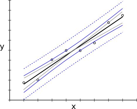
Figure 1 illustrates this by the presence of one regression line (black) and two other lines (both gray) not being statistically significantly different from the regression line. They are thus also potential candiates for the true regression line. All three lines are contained within the confidence band (blue solid lines).
 -percent confidence band contains the true regression curve with
  percent confidence.
At a given predictor value  (small dots), the upper- and lower confidence value basically build the confidence interval for the mean value / regression curve value
  at this point.
By the way, the confidence band for a given data set gets broader if a higher confidence level is needed. For instance, if 99 % confidence is required the corresponding confidence band will be broader (along y) compared to the 95 % confidence band. That might seem a bit counterintuitive but in these cases I tend to think of Gaussian distributions centered around the experimental regression curve at the corresponding predictor values and whose width are primarily determined by the uncertainty of the fit parameters and the predictor values. Try to think of the lower (i.e.  ) and upper quantiles (i.e.
  ) of these distributions and you end-up with outer regions of the confidence intervals. E.g. if you think of the 2.5 % lower and 97.5 % upper quantile, you end-up with 95 % confidence intervals. However, if you choose the 0.5 % and 99.5 % quantiles, you end-up with 99 % confidence intervals. The area of the distributions limited by the quantiles is bigger in the latter case than in the former one. That means the corresponding confidence intervals are broader. When I talk about certain predictor values, I use the terminology confidence intervals, but when I talk about a confidence band, I mean the continous set of confidence intervals along all predictor values. Please note that the Gaussian distributions that I just talked about and which are displayed in figure 2, do not represent the variability of the data.

There is another common type of band plotted around the actual fit curve, namely the prediction band. Prediction bands are like confidence bands but additionally take the variability of the data around the fit curve into account. Thus, prediction bands are always broader than confidence bands (see dashed lines in figure 1).
Here is the second core message in this post:
Future data points will fall within the prediction band region with a probability of .
Please note that while the width of confidence band is determined by the uncertainty of the fit parameters and by the predictor values, the width of the prediction band is mostly determined by the variability of the data itself. While increasing the number of data points makes the fit parameter estimates better and better, and thus reduces the width of the confidence band, this is not equally true for the prediction band. This is simply because the variance of the data does not really change if additional data points arise and so does not change the prediction band width. If the influence of variability of fit parameters becomes negligible, the prediction band outer regions approach a constant distance away from the regression line, independent of the corresponding predictor values (given that the data is homoscedastic).
At this point I should probably mention that there are various methods how confidence intervals / bands can be calculated. The method that I had in mind when writing this blog post is referred to as asymptotic approximation. Confidence intervals computed by this method are often referred to as asymptotic confidence intervals (you can easily find more details on Google). The asymptotic approximation method is the one which is most often implemented in various statistical software packages. Other methods are based on bootstrapping, Monte-Carlo methods or based on the so-called profile-likelihood method which shall not be covered in this post.
Simultaneous or non-simultaneous? What is that?
To fully understand the concept behind simultaneous confidence or prediction bands, we would need to talk about the concept of multiple comparisons first. However, here we will not go into so much detail since this topic will anyway be covered in future blog post. But for now, it is sufficient to know that simultaneous confidence or prediction bands are typically broader than their corresponding non-simultaneous counterparts. This is because the significance level and correspondingly the confidence level is adjusted in a way that a collection of confidence intervals (at all predictor values) cover the true regression curve with 95 % confidence (I will leave prediction bands aside here, but the same logic applies here, too). If you would only look at non-simultaneous confidence intervals (sometimes referred to as single confidence intervals) this confidence level would only apply to each single interval. Fitting many data sets , simulated from a known fit model and with normally distributed random noise added, can help to get a feeling for the difference between simultaneous and non-simultaneous confidence and prediction bands, respectively. In these simulations the true regression curve is known and one can for instance check how often this true regression curve is fully contained within the non-simultaneous confidence bands of the fitted regression curves. This will be less than 95 % of the time since for each specific predictor value the probability that the corresponding data point of the true curve is within the confidence interval at is 95 %. Thus, the probability that at least one protrudes out of range increases with the number of single confidence intervals. To circumvent this with simultaneous confidence intervals, the confidence level is adjusted using methods well-known from multiple comparison, like Bonferroni, Tukey, Sidak, just to name a few. Some of these methods will be discussed elsewhere.
Confidence bands are often used to estimate the uncertainty of interpolated predictor-values. E.g. if a regression curve was created by measuring standards of known concentrations (signal on y-axis, concentration on x-axis) then the unknown concentrations of samples can be estimated by interpolating their corresponding concentrations from the signal and the fitcurve (see figure 3). The uncertainties associated with the concentration estimates, expressed in terms of confidence intervals, can be estimated by interpolating from the signal values and the confidence band. Please note that these estimated confidence intervals are typically asymmetric.
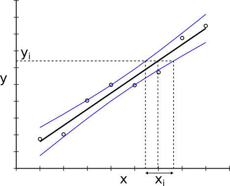 obtained by interpolating from the confidence band.