Demystifying the Hill Equation for Assay Developers

The Hill-model and similar ones are often used in the fields of drug discovery to model experimental data from dose-response-, binding- or bioassays. In this blog post I will try to shed light on what the hill model actually is and on the confusing terminology that occurs with respect to the Hill and other models used to model the aforementioned kind of data.

When you take a course on physical chemistry, you’ll likely be confronted with the concepts of adsorption isotherms, especially with the model derived by Langmuir. This model can be used to describe the adsorption or gasoues molecules to single-layered binding sites. But it can also be used to describe the adsorption of dissolved molecules to solid monolayeric binding sites.

I was surprised to hear that the concept of this type of biniding had even been published a few years earlier by the physiologist and
pharmacologist A.V. Hill and today is often referred to as Hill equation:

\theta = \frac{K \cdot [S]^n}{1 + K \cdot [S]^n}

where:

$\theta$ is the fraction of binding sites occupied,
$[S]$ is the concentration of the sorbent,
$n$ is the Hill coefficient (a measure of cooperativity),
$K$ is an equilibrium constant.

The parameter $n$ is known as Hill coefficient or Hill slope and is a measure of cooperativity of binding. A positive cooperativity $n > 1$ means that already bound molecules increase the binding affinity of free molecules while a negative cooperativity indicates that already bound molecules reduce the affinity of free molecules to bind to the target.

For $n=1$ the binding of molecules to the target does not influence the binding of other molecules to the target.

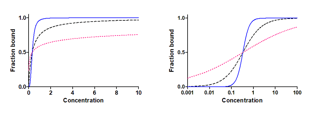Left: The modified Hill equation (see section “The Hill equation in a new guise”) plotted on a linear concentration scale for $n=1$ (black dashed line), $n=3$ (blue solid line) and for $n=1/3$ (red dashed line).
Right: The same data as left but plotted on a semilogarithmic concentration axis.

For $n=1$ the Hill equation becomes the equation derived by Langmuir for the adsorption of ideal gas molecules:

\theta = \frac{n_a}{n_{max}} = \frac{K \cdot [S]}{1 + K \cdot [S]}

where $n_a$ and $n_{max}$ denote the amount of adsorbed and maximal possible amount of molecules on the monolayer, respectively. Here, $K$ denotes the Langmuir constant being equal to the ratio of adsorption to desorption constant: $K = \frac{k_{ads}}{k_{des}}$

In general, the Hill equation describes a hyperboloid shape. For $n=1$ it describes a classical hyperbola while for $n>1$ it becomes more and more sigmoid when plotted against a linear concentration scale (see figure above). In practice, however, it is quite common to use a semilogarithmic concentration axis so that all of these curves become sigmoid. I want to point out the similarity (in fact equality for $n=1$ ) between the Hill equation and the well-known Michaelis-Menten model used to fit experimental data from simple enzyme kinetic assays and published 3 years after Hill’s paper from 1910:

y = \frac{v}{v_{max}} = \frac{[S]}{K_M + [S]} = \frac{\frac{1}{K_M}[S]}{1+\frac{1}{K_M}[S]} = \frac{K \cdot [S]}{1 + K \cdot [S]}

where we have defined $K \equiv 1/K_M$ being the inverse of the Michaelis-Menten constant.

The Hill equation in a new guise

In the literature you’ll find various equations related to the term ‘Hill’. Hill equation, logistic-Hill equation, logit Hill and so on. The equation stated at the beginning of this blog post is the one originally published by Hill in 1910. However, the more common form is the following, slightly modified version of the Hill equation:

\theta = \frac{K_a^n \cdot [S]^n}{1 + K_a^n \cdot [S]^n} = \frac{1}{1 + \frac{1}{\left(K_a \cdot [S] \right)^n}}

$K_a$ now denotes an association constant and — taken to the power of the Hill coefficient $n$ — replaces the apparent equilibrium dissociation constant $K$ of the original Hill equation resulting in the modified Hill equation just stated. The right hand side of the last equation is an algebraically simplified version of the modified Hill eqaution that will be helpful later on.

For any $K_a$ the modified Hill model asymptotically approaches 1 for increasing concentrations. As Hill was working on Haemoglobin multimerization and oxygen saturation, his experimental response could at max approach 100 percent (saturation). In practice, however, the upper asymptote could be different from 1. In this case the modified Hill equation is extended:

y = \theta_{max} \frac{K_a^n \cdot [S]^n}{1 + K_a^n \cdot [S]^n}

where $\theta_{max}$ denotes the upper asymptote that the experimental readout approaches to at high concentrations [S]. The last equation is sometimes referred to as 3-parameter Hill equation. In addition, there might be a non-zero response when the concentration $[S]$ approaches zero, so to say a baseline response. In this case we need to extend the last equation even further to account for this:

y = \left(\theta_{max} – \theta_{min} \right) \frac{K_a^n \cdot [S]^n}{1 + K_a^n \cdot [S]^n} + \theta_{min}

We can now we write the often-called 4-parameter Hill equation in a form that is quite commonly seen in literature:

y = \frac{\theta_{max} – \theta_{min}}{1 + \frac{1}{\left(K_a \cdot [S] \right)^n}} + \theta_{min} = \frac{\theta_{max} – \theta_{min}}{1 + \left(\frac{\tilde{K}}{[S]}\right)^n} + \theta_{min}

Here, I replaced $1/K_a$ by $\tilde{K}$ . In dose-response analysis $\tilde{K}$ is typically called the $ED_{50}$ (effective dose 50) or $EC_{50}$ (effective concentration 50). For inhibitory assays it is called $IC_{50}$ (inhibitory concentration 50). They all indicate the concentration/dose at half maximum response, a useful measure for comparing the effectiveness of drugs for example.

When you try to fit that dose-response curve model to your experimental data, you might sometimes recognize convergence issues resulting in parameter estimates that might be non-optimal. This is especially problematic when you are the one to provide initial guess values for the curve fitting routine. It is easier to guess fit parameters ( $\theta_{min}$ , $\theta_{max}$ , $\tilde{K}$ and $n$ ) as starting point for the fit from the semilogarithmic dose-response plot. Furthermore, there are statistical reasons why at least a semilogarithmic transformation of the concentration values makes sense (for more details, see the book ‘Fitting models to biological data using linear and nonlinear regression’ by Motulsky and Christopoulos). As a result, the often-called logistic-Hill equation is routinley fitted to dose-response data:

y = \frac{\theta_{max} – \theta_{min}}{1+\exp\left(- n \cdot \left(\log([S] – \log(\tilde{K})) \right) \right)} + \theta_{min}

with $\log$ being the natural logarithm and $\exp()$ denoting the exponential function. If doses are based on tenfold serial dilution it is also common to use $\log10$ instead of $\log$ and take to the power of base 10 instead of the exponential function:

y = \frac{\theta_{max} – \theta_{min}}{1+10^{\left(- n \cdot \left(\log10([S] – \log10(\tilde{K})) \right) \right)}} + \theta_{min}

The last two equations are often called 4-parameter logistic or logistic 4-parameter instead of logistic 4-parameter Hill equation. But again, there is no consistent terminlogy in the literature and in different statistical software packages.

We have now seen a lot of different variants and terminology around the Hill equation. During discussions with scientists it often turns out that people relate different formula with “the” Hill equation. And this can be very confusing and misleading.

Let’s make things even more complex and introduce the generalized for of the Hill equation, also known as Richard’s function:

y = \frac{\theta_{max} – \theta_{min}}{\left(1 + \left(\frac{\tilde{K}}{[S]}\right)^n\right)^a} + \theta_{min}

or in its logistic form:

y = \frac{\theta_{max} – \theta_{min}}{\left(1+10^{\left(- n \cdot \left(\log10([S] – \log10(\tilde{K})) \right) \right)}\right)^a} + \theta_{min}

It accounts for asymmetry of the dose-response curve. But being able to fit this model to experimental data requires qualitatively good data and again, useful initial guess values. For the latter equation you’ll find other names in the literature like 5-parameter logistic or logistic 5-parameter.

In this blog post I tried to unvravel things a bit. When publishing results derived from these models, good scientific practice requires including the exact mathematical equation used for data fitting, along with any preprocessing steps such as data transformations.

If you need to fit your experimental dose-response or binding data to a Hill model yourself, try out the Biotfitting-App on our software page. You can choose from different fit models including the 4-parameter and 5-parameter logistic equation mentioned above.