Finding roots and Hunting for an Optimum

In process control it is a common goal to maximize the yield of a product by finding the optimal process parameters. In a bioreactor for instance, parameters like temperature, nutritional supplementation and pH are optimized to grow bacteria under ideal conditions, e.g. to maximize the yield of a metabolic product. A more mathematical example includes regression analysis where the sum-of-squared errors are minimized with respect to fit model parameters which means that the corresponding derivative w.r.t the fit parameters are set to zero. In a general setting that means finding the roots of a system of equations. Root finding algorithms are indispensible tools in optimization problems and frequently applied in science and engineering. In this blog post we will discuss two common root-finding methods, the bisectioning method and the Newton-Raphson method and I’ll demonstrate how use LAMBDA-functions to create corresponding functions in Excel.

The Newton Method: A Swift and Efficient Approach

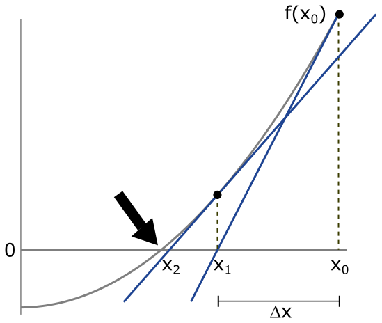
The Newton method is a powerful iterative technique, leveraging the concept of tangent lines to approximate the roots of a function. The process is as follows:

Initial Guess: We start with an initial guess, denoted as $x_0$ .
Tangent Line: A tangent line is drawn to the function’s curve at the point $\left(x_0, f(x_0)\right)$ .
Next Approximation: The $x$ -intercept of this tangent line becomes the next approximation, $x_1$ .
Iteration: The process is repeated, using $x_1$ as the new initial guess.

Let’s mathematize this a bit more and express the whole iteration in one line:

$x_{i+1} = x_i - \frac{f(x_i)}{f'(x_i)}$

Where does this formula come from? The basic idea behind the Newton-Raphson method is to approximate the actual function $f(x)$ near $x_0$ by a tangent having slope $f'(x_0)$ , and to solve for the root $x_1$ of that tangent, i.e. the point where the tangent crosses the $x$ -axis. This crossing point $x_1$ is a better approximation to the actual root of the function and is used in the next iteration. There, $x_1$ is plugged into the derivative function $f'(x_1)$ that is used as the slope of a new tangent. Again, the root $x_2$ of that tangent is found and used in the next iteration. This process is repeated until there is no noticeable change in successive $x$ -values. Then a root is found (arrow in figure below).

Note that at iteration $i+1$ , $x_{i+1}$ and the former $x_i$ are seperated by $\Delta x$ , i.e. $x_{i+1} = x_i - \Delta x$ . Looking at the tangent that passes through $\left($ x_{i+1} $, 0\right)$ and $\left($ x_i $, f(x_i)\right)$ , the slope is given by:

$f'(x_i) = \frac{f(x_i) - 0}{\Delta x} = \frac{f(x_i) }{\Delta x}$

Solving for $\Delta x = x_i - x_{i+1}$ and by rearranging for $x_{i+1}$ we get the equation (as before):

$x_{i+1} = x_i - \frac{f(x_i)}{f'(x_i)}$

So it is a quite basic but powerful algorithm that is often used in practice. Excel’s Goal Seek and the Solver both apply the Newton-Raphson method. However, these tools do not dynamically update results when corresponding cells change and the re-calculation needs to be triggered manually. One way to update results dynamically is to create your own LAMBDA-function that does the calculations for you. Find a corresponding code below:

=LAMBDA(f,df,x0,i,[tol],[max_iter],
  LET(
    tol, IF(ISOMITTED(tol), 0.001, tol),
    max_iter, IF(ISOMITTED(max_iter), 200, max_iter),
    x, x0,
    iter, 0,
    output, LAMBDA(x,iter,
      LET(
        fx, f(x),
        dfx, df(x),
        x_new, x - fx / dfx,
        IF(
          OR(ABS(fx) < tol, iter >= max_iter),
          x_new,
          NEWTONRAPHSON(f,df,x_new, iter + 1, tol, max_iter)
        )
      )
    ),
    output(x, iter)
  )
)

Make sure to create this function in Excel’s Name Manager, Therefore, open the Name Manager from the Fomulas menu and paste the code above in the Refers to: section. Assign NEWTONRAPHSON to the Name of the function. Afterwards you can apply this to your own root-finding problems.

Note that the success of the Newton-Raphson method very much depends on the initial guess. Especially is a function like $f(x)=x^2-4$ has two or more roots, the particular choice of $x_0$ determines which root will be found first.

The Bisection Method: A Steady and Reliable Approach

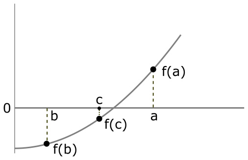
The bisection method, a more straightforward technique, involves repeatedly dividing an interval in half and selecting the subinterval that contains the root. The steps are as follows:

Iteration: The process is repeated with the reduced interval.

Interval Selection: We start with an interval [a, b] where the function changes sign.

Midpoint Calculation: The midpoint, c, is calculated as (a+b)/2.

Interval Reduction:

If f(c) = 0, c is the root.
If f(a) and f(c) have opposite signs, the root lies in [a, c].
If f(b) and f(c) have opposite signs, the root lies in [c, b].

If you are a MATLAB enthusiast, you might know the fzero function that does apply this bisectioning approach to find the roots of nonlinear functions. Below you find the corresponding LAMBDA-function that does the job for you in Excel:

=LAMBDA(f, a, b, [tol],
  LET(
    tol, IF(ISOMITTED(tol),0.001,tol),
    fa, f(a),
    fb, f(b),
    mid, (a + b) / 2,
    fmid, f(mid),
    IF(
      ABS(fmid) < tol, 
      mid, 
      IF(
        SIGN(fa) = SIGN(fmid), 
        BISECTION(f, mid, b, tol), 
        BISECTION(f, a, mid, tol)
      )
    )
  )
)

As before, make sure to create this function in Excel’s Name Manager, Therefore, open the Name Manager from the Fomulas menu and paste the code above in the Refers to: section. Assign BISECTION to the Name of the function. Afterwards, you can apply this to your own root-finding problems.
Simililar to the Newton-Raphson method, the convergence of the Bisection method depends on the particular choice of $a$ and $b$ . These shouldn’t be too far from the actual root.

So if you have absolutetly no idea what the root(s) might be, it can be difficult to find them. But you should at least play around with the intial guess values and see if in multiple runs there is a convergence towards certain values that are then likely your roots.

One advantage of using the Bisection method over the Newton-Raphson is that it does not require calculating the derivative of the function. The Newton-Raphson, however, does require either an analytical or numerical derivative of the function. Unfortunately, the analytical derivative is often not tractable or hard to compute. In this case one could use a forward difference scheme like $\frac{f(x+\Delta x)-f(x)}{\Delta x}$ as an approximation to the derivative. I’ve adapted the Newton-Raphson code from above to cases, where there is no analytical derivative available (see code below).

=LAMBDA(f,x0,i,tol,max_iter,
  LET(
    tol, IF(ISOMITTED(tol), 0.001, tol),
    max_iter, IF(ISOMITTED(max_iter), 200, max_iter),
    x, x0,
    dx, 0.001,
    iter, 0,
    output, LAMBDA(x,iter,
      LET(
        fx, f(x),
        dfx, (f(x+dx)-fx)/dx,
        x_new, x - fx/dfx,
        dx, x-x_new,
        IF(
          OR(ABS(fx) < tol, iter >= max_iter),
          x_new,
          NEWTONRAPHSON(f,x_new, iter + 1, tol, max_iter)
        )
      )
    ),
    output(x, iter)
  )
)

Finding roots and Hunting for an Optimum

Dr. Mario Schneider

Leave a Reply Cancel reply

Data analysis for scientists,
engineers and practitioners