The Savitzky-Golay Method: Smoothing and Differentiating Experimental Data

The first time I came across smoothing with the Savitzky-Golay method was during my chemometrics class at university analyzing spectroscopy data using chemoetric methods. And indeed, the Savitzky-Golay method seems to have quite some awareness among spectroscopist, probably because Savitzky and Golay also worked in this field and referred to spectroscopy in their paper in 1964. The Savitzky-Golay method seems like one of those methods — similar to the moving average — where a sliding window of defined size is slid over the data and each time the smoothed version of the point $\hat{y}_k$ is calculated by averaging all data points inside the current window. In contrast to the moving average, the Savitzky-Golay method applies a sort of weighted average instead. But there is more to it as we shall see in this blog post.

$\hat{y}_k = \frac{\sum_{i=k-m}^{k+m}c_i y_i}{\sum_{i=k-m}^{k+m}c_i}$

The $c_i$ ‘s are the weights and denote the Savitzky-Golay coefficients. These are tabulated for various window sizes $2m+1$ (an excerpt of such a table is shown below).

	Window size = 5	Window size = 7	Window size = 9
$c_{-4}$			-21
$c_{-3}$		-2	14
$c_{-2}$	-3	3	39
$c_{-1}$	12	6	54
$c_0$	17	7	59
$c_1$	12	6	54
$c_2$	-3	3	39
$c_3$		-2	14
$c_4$			-21

It is common practice to use generalized data point indices in these tables, i.e. the central point of the sliding window has the index 0, while its direct left neighbour gets index -1 and its direct right neighbour +1 etc.

E.g. for a window size of 5 the 3rd data point of the smoothed signal is calculated by:

$\hat{y}_3 = \frac{\sum_{i=3-2}^{3+2}c_i y_i}{\sum_{i=3-2}^{3+2}c_i} = \frac{-3y_1 + 12y_2 + 17y_3 + 12y_4 - 3y_5}{35}$

Then the sliding window is shifted one data point index upwards with $y_4$ as the new center and the calculation is repeated with the new 5 data points inside that new window. And so on. This whole process can mathematically be expressed as a convolution:

$\hat{y} = C \otimes y$

where $y$ denotes the original signal and $C$ denotes the convolution kernel, i.e. the vector of filter coefficients.

Boundary points (1, 2 and N-1, N for a window size of 5) must be treated differently as they do not have enough neighbouring data poinst left and right, respectively. Without digging too deep: one approach is to use the 2m+1 neighbourhood closest to the boundary point and fit these with a polynomial of appropriate size and estimate the boundary ordinate from the polynomial. Another approach is to use dedicated weight coefficients for the boundary points as described by Gorry in 1990.

Interestingly, when plotting the $c_i$ ‘s from the table above in a chart, you will realize that they form a parabola. Thus, the Savitzky-Golay is similar to the moving average but instead of a uniform weighting of data points inside the sliding window, the Savitky-Golay method applies a parabolic, or more general, a polynomial weighting.

The original paper by Savitzky and Golay in 1964 is very informative as they show that the convolutional approach with the coefficients $c_i$ naturally derives from fitting a polynomial $p(n)$ to a general sliding window with data points $n \in \{-M,...0,...,M\}$ :

$p(n) = \sum_{k=0}^{N} a_k n^k = a_0 + a_1 n + a_2 n^2 + a_3 n^3 + \dots$

and estimating the center point $p(0)$ of that interval from the polynomial approximation at that position. At the end of this blog post I will sketch the derivation for the math-affine readers.

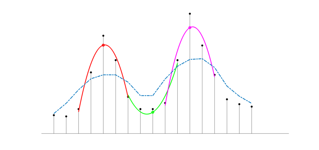
The following chart demonstrates the polynomial fitting for a discrete signal (black dots) with two peaks, one with a maximum at index 5 and another one with a maximum at index 12 and a valley in betwen the peaks. Examplarily, three sliding windows of size 5 were fitted each with a quadratic polynomial (red, green and magenta lines) and the center points (denoting the smoothed signal) are highlighted by circles of the same color. For reference, I added a moving average line (dash-dotted blue line) smoothed on the same window size, demonstrating that the Savitzky-Golay preserves the peak shape reasonably well while the moving average smoothes much coarser.

The advantage of the convolutions over the polynomial fitting approach is that the convolution approach is faster as it does not require to fit new polynomial coefficients to each sliding window but applies fixed Savitzky-Golay coefficients depending only on the sliding window width and the degree of the polynomial.

Another nice thing about the Savitzky-Golay method is its use for calculating derivatives of signals. Noisy signals must typically be smoothed ahead of taking their derivative. In these cases it is a two-step process: smooth first, then take the derivative. With Savitzky-Golay you can skip the first step as a dedicated set of SG-coefficients applies both at the same time: smoothing and derivation.

In the following I summarize some core features of smooting or derivating with the Savitzky-Golay filter:

Smoothing

Because it fits a polynomial (usually of degree 2, 3, or 4) rather than a straight line, it is exceptionally good at preserving the height, width, and shape of spectral peaks while reducing high-frequency noise.
The degree of smoothing depends on the window size (larger windows = smoother data) and the polynomial order (higher order = better feature preservation but less noise reduction).

Differentiation

One of the most powerful features of the SG filter is its ability to calculate derivatives directly from the smoothing process.
Standard finite-difference methods amplify noise significantly. SG differentiation acts as a “differentiator-smoother,” providing a much cleaner derivative signal.
In spectroscopy, the second derivative is frequently used to resolve overlapping peaks; SG allows for this without losing the underlying signal structure.

A note of caution: The SG filter can be a great tool but when smoothing signals of high variability (e.g. different Peaks with different widths) a single parameter combination of window size and polynomial degree might be inappropriate. In fact, this is still an area of research on how to deal with these kinds of situations. Techniques like adaptive SG smoothing have been developed for this purpose.

I provide this Excel file that contains the custom SGOLAYFILT function that can smooth or differentiate a signal based on the Savitzky-Golay method.

For those interested in the maths

In this section I’ll give a brief and hopefully more appealing derivation of the Savitzk-Golay coefficients than in their own paper. We begin by considering $2m+1$ sample points $-M, \dots, 0, \dots, M$ centered at $n=0$ . We fit a polynomial $p(n) = \sum_{k=0}^{N}a_k n^k$ to the underlying data: $y_{-M}, \dots, y_0, \dots, y_M$ in a least-square sense, i.e. by minimizing the sum-of-squared error (SSE) between the data points and their polynomial correspondents wrt the polynomial coefficients $a_k$ :

$\min_{a_0,\dots, a_N} \sum_{n=-M}^{M}\left(\sum_{k=0}^{N} a_k n^k - y_n\right)^2$

To keep the notation simple, we’ll use the following vector/matrix notation instead:

$\min_{a_0,\dots, a_N} \left(\mathbf{\hat{y}} - \mathbf{y}\right)^T \left(\mathbf{\hat{y}} - \mathbf{y}\right)$

where $\mathbf{y} = \left[y_{-M}, \dots, y_0, \dots, y_M \right]$ and $\mathbf{\hat{y}} = \mathbf{J}\mathbf{a}$ , with $\mathbf{J}$ being the so-called Vandermonde matrix, with entries:

$\mathbf{J} = \left[\mathbf{j}_0, \mathbf{j}_1, \dots, \mathbf{j}_N \right]$

where $\mathbf{j}_k = n^k$ is a column vector (with $n$ ranging from $-M$ to $M$ ) and $\mathbf{a}$ being the the polynomial coefficients from above. For example $\mathbf{j}_0$ is a column vector of ones ( $k=0$ ), $\mathbf{j}_1$ a column vector of $[-M, \dots, 0, \dots, M]^T$ (for $k=1$ ), $\mathbf{j}_2$ a column vector of $[M^2, \dots, 0, \dots, M^2]^T$ (for $k=2$ ) and so on.

Plugging $\mathbf{\hat{y}} = \mathbf{J}\mathbf{a}$ into the expression for the sum-of-squared error we re-formulate the minimization problem as follows:

$\min_{a_0,\dots, a_N} \left(\mathbf{J}\mathbf{a} - \mathbf{y}\right)^T \left(\mathbf{J}\mathbf{a} - \mathbf{y}\right)$

From the above equation we can solve for the polynomial coefficients $\mathbf{a}$ using matrix algebra (e.g. see our blog post on weighted regression):

$\mathbf{a} = \left(\mathbf{J}^T\mathbf{J}\right)^{-1} \mathbf{J}^T \mathbf{y}$

From the fact that our model is linear in its coefficients we can express the smoothed signal by:

$\mathbf{\hat{y}} = \mathbf{J} \mathbf{a} = \mathbf{J} \left(\mathbf{J}^T\mathbf{J}\right)^{-1} \mathbf{J}^T \mathbf{y}$

The matrix $\mathbf{H} \equiv \mathbf{J} \left(\mathbf{J}^T\mathbf{J}\right)^{-1} \mathbf{J}^T$ has size $(2M+1) \times (2M+1)$ and is often called the hat matrix. It is interesting to note that the entries in $\mathbf{H}$ are independent of the samples and only depend on the length of the sliding window and on the polynomial order chosen. By the last equation we approximate each point in the window $-M,\dots, 0, \dots, M$ by the polynomial defined by its coefficients in $\mathbf{a}$ . But in fact, only the central point at $n=0$ shall be approximated. so that only the $M+1$ th row vector of the hat matrix is required to calculate the smoothed center point of the sliding window. Let’s call this vector $\mathbf{h}_0$ . The Savitzky-Golay coefficients correspond to the entries in $\mathbf{h}_0$ . Extract the corresponding row vector by multiplying the $1 \times (2m+1)$ -vector $\left[0, \dots, 0, 1, 0, \dots, 0 \right]$ with the hat matrix $\mathbf{H}$ . By the way, the same coefficients you would have also gotten from the first row of the matrix $\mathbf{B} \equiv \left(\mathbf{J}^T\mathbf{J}\right)^{-1} \mathbf{J}^T$ which would require one less matrix multiplication. $\mathbf{B}$ is also used when it comes to calculating derivatives. The second row of $\mathbf{B}$ corresponds to coefficients used to calculate the first derivative at the center point. Or more general, the $d$ -th derivative corresponds to the $(d+1)$ -th row in $\mathbf{B}$ scaled by a factor $d!$ and divided by $T^d$ (given the spacing between data points is not $T=1$ ).

I guess after so much theory a short example will clarify things a bit.

Example

Say we have a window width of $2M+1 = 5$ , so the data points $-M, -(M-1), \dots, 0, \dots, M-1, M$ are equal to $-2, -1, 0, 1, 2$ . Thus, for a polynomial for degree 2 we can write down the matrix $\mathbf{J}$ as:

$\mathbf{J} = \begin{bmatrix}1 & -M & M^2 \\1 & -(M-1) & (M-1)^2 \\\vdots & \vdots & \vdots \\1 & M & M^2\end{bmatrix} = \begin{bmatrix}1 & -2 & 4 \\1 & -1 & 1 \\1 & 0 & 0 \\1 & 1 & 1 \\1 & 2 & 4\end{bmatrix}$

Calculating $\mathbf{H}$ returns in this example:

$\mathbf{H}_{5 \times 5} = \frac{1}{35} \begin{bmatrix}31 & 9 & -3 & -5 & 3 \\9 & 13 & 12 & 6 & -5 \\\mathbf{-3} & \mathbf{12} & \mathbf{17} & \mathbf{12} & \mathbf{-3} \\-5 & 6 & 12 & 13 & 9 \\3 & -5 & -3 & 9 & 31\end{bmatrix}$

I highlighted the central row vector $\mathbf{h_0}$ in bold. Compare its entries with the entries in table from the beginning and you’ll see the coefficients equivalence.

The matrix $\mathbf{B}$ is in this example:

$\mathbf{B}_{3 \times 5} = \frac{1}{35} \begin{bmatrix}-3 & 12 & 17 & 12 & -3 \\-7 & -3.5 & 0 & 3.5 & 7 \\5 & -2.5 & -5 & -2.5 & 5\end{bmatrix}$

Literature

A. Savitzky and M. J. E. Golay, Smoothing and differentiation of data by simplified least squares procedures, Anal. Chem., vol. 36, pp. 1627–1639, 1964.

Gorry, P. A. General least-squares smoothing and differentiation by the convolution (Savitzky-Golay) method. Anal. Chem. 1990, 62, 570−573.

Schafer, R. W. What is a Savitzky-Golay filter? [Lecture Notes]. IEEE Signal Processing Magazine 2011, 28, 111−117.

Savitzky-Golay Filter article on Wikipedia: https://en.wikipedia.org/wiki/Savitzky%E2%80%93Golay_filter